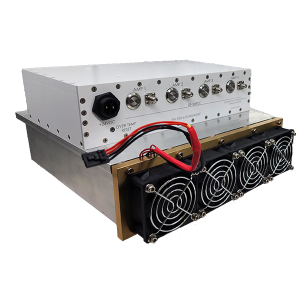
The catalog part looks perfect on paper. The noise figure is within spec, the gain is adequate, the package fits the board, and the lead time is four weeks. Six months into the program, the system is 3 dB short of its sensitivity requirement, two radar modes are failing their acceptance tests, and nobody can explain why – until someone runs a full thermal and impedance analysis at the assembly level and finds that three assumptions embedded in the catalog datasheet simply do not hold under the actual operating conditions.

This scenario is not unusual in millimeter wave hardware development. The gap between what a catalog mmWave amplifier datasheet guarantees and what that same device delivers when integrated into a real subsystem – at temperature, under realistic source and load impedances, in proximity to adjacent components on a dense assembly – is wider than most engineers account for during component selection. At microwave frequencies below 20 GHz, these discrepancies are often small enough to absorb. Above 50 GHz, they frequently determine whether a system passes or fails.

This article examines the specific ways catalog mmWave amplifiers mislead experienced engineers, the conditions under which custom mmWave amplifiers become the correct engineering choice, and the questions that should inform every amplifier selection decision above 30 GHz.

What Catalog Datasheets Do Not Tell You

Impedance Match: The 50-Ohm Fiction

Every mmWave amplifier datasheet specifies gain, noise figure, and output power referenced to a 50-ohm source and load impedance. This is a measurement convention, not a description of the device’s actual impedance environment. The input and output reflection coefficients (S11 and S22) tell you how closely the device matches 50 ohms, but in a real system, the source driving the amplifier input is a mixer, a filter, an antenna feed, or the output of another amplifier – none of which present exactly 50 ohms at the operating frequency.

At Ka-band (26.5–40 GHz) and above, a mismatch that appears minor in a datasheet produces a significant gain and noise figure variation when the actual source impedance deviates from 50 ohms. The noise figure of a low-noise amplifier in particular is extremely sensitive to source impedance. The minimum noise figure specified on a datasheet is achieved only at a specific optimum source impedance, which is never exactly 50 ohms. The noise figure actually achieved in a real system with a non – 50-ohm source impedance can be substantially higher than the datasheet value suggests.

Custom mmWave amplifiers are designed with knowledge of the actual source and load impedances in the intended signal chain. The input matching network is optimised for the true source impedance of the preceding component – whether a waveguide filter, a horn antenna feed, or a mixer output – and the result is a device that performs to specification in the real system rather than in a characterisation fixture.

Noise Figure vs. System Noise Temperature

Catalog low – noise amplifier noise figures are measured at room temperature with a calibrated noise source. In deployed systems, the physical temperature of the amplifier module varies with ambient conditions, thermal dissipation of adjacent components, and duty cycle. The noise figure of a precision low-noise amplifier typically increases by 0.3–0.5 dB across the operating temperature range – a variation that directly degrades receiver sensitivity and is absent from most catalog datasheets, which specify noise figure at a single temperature point.

For systems with a demanding noise budget – radar receivers targeting specific minimum detectable signal levels, radiometers, or communications systems operating at link margin limits – this thermal variation cannot simply be absorbed. It must either be managed through thermal design or accounted for in the noise budget with explicit worst-case margin. Catalog parts rarely provide the characterised noise figure versus temperature data needed to do this analysis rigorously.

Gain Flatness Over Frequency and Temperature

Wideband radar and EW receivers require the amplifier chain to maintain consistent gain across the operating bandwidth. A catalog amplifier specified with plus or minus 1.5 dB gain flatness across a 10 GHz bandwidth may have its gain variation concentrated at specific frequencies – frequencies that happen to coincide with the radar’s primary operating modes. Without access to detailed S-parameter files and statistical characterisation data across production lots, the engineer has no way to predict or control this.

Custom mmWave amplifiers, particularly those developed through a matched amplifier design process, can be optimised for gain flatness across a specified band as an explicit design objective, with production test limits enforcing that specification across every device shipped. Low-noise, power, driver, and variable gain amplifiers covering X – band through W-band, when specified and characterised for gain flatness as a primary parameter, deliver the signal chain consistency that catalog parts cannot guarantee.

When the Gap Between Catalog and Custom Becomes Critical

Cascaded Noise Figure in Long Receive Chains

The Friis noise figure formula establishes that the noise figure of a cascade is dominated by the first stage, with each subsequent stage contributing less as the gain preceding it increases. This makes the selection of the first low – noise amplifier in a receive chain by far the most important amplifier decision in the entire signal chain. At mmWave frequencies, where a catalog amplifier might specify 3 dB noise figure but deliver 4.5 dB in the actual circuit due to source impedance mismatch and thermal effects, the entire cascade noise figure budget can be exceeded before the second stage is even considered.

Custom mmWave amplifiers designed for the first stage of a specific receive chain – optimised for the true source impedance of the antenna feed or waveguide component that precedes them, characterised for noise figure across operating temperature, and matched to the filter or mixer that follows – routinely achieve 0.5–1.0 dB better noise figure in situ than the best available catalog amplifier at the same frequency. In systems where every fraction of a dB in noise figure translates directly to detection range or link margin, this difference is not marginal.

Harmonic and Spurious Performance in EW Transmitters

Electronic warfare transmitters have strict spurious emission requirements. A catalog power amplifier specified for output compression point and third-order intercept may meet those specifications in a 50 – ohm test setup but produce substantially higher harmonic content when the output is connected to a real antenna through a transmission line with frequency-dependent impedance. The harmonic levels at the antenna port – the ones that matter for electromagnetic compatibility compliance – are determined by the combination of the amplifier’s nonlinear characteristics and the impedance it sees at harmonic frequencies, not just its two-tone intermodulation performance in a test fixture.

In EW system development, discovering that harmonic levels fail military conducted emissions specifications late in the integration phase – when the antenna, feedline, and amplifier are all fixed – is a costly program risk. Custom mmWave amplifiers designed with the actual output impedance environment characterised across fundamental and harmonic frequencies allow the harmonic performance to be engineered as part of the matching network design rather than discovered by accident during system integration.

SWaP-Constrained Designs

Airborne and missile seeker platforms impose strict size, weight, and power constraints that catalog amplifier packages frequently cannot meet. A catalog amplifier in a standard package with a fixed decoupling topology may consume more assembly area or require more bypass components than the module can accommodate. Custom mmWave amplifiers implemented as bare die assemblies, chip-and-wire modules, or integrated multi-function packages combine gain, matching, biasing, and power management in a form factor sized to the available volume – something no catalog product can offer. This is particularly relevant for compact front-end components supporting systems from X – band through W-band in defense and aerospace applications.

What Engineers Should Ask Before Selecting Any mmWave Amplifier

Whether evaluating catalog parts or initiating a custom development, the following questions should be answered before committing to an amplifier selection above 30 GHz:

• What is the actual source impedance driving the amplifier input, and how does it vary across the operating band? Has the noise figure been evaluated at that impedance, not just at 50 ohms?
• What is the amplifier’s junction temperature under worst-case dissipation conditions, and how does noise figure, gain, and output compression point vary across that temperature range?
• Are statistical S-parameter and noise parameter files available from the manufacturer, or are only nominal typical and minimum/maximum datasheet values provided?
• What is the amplifier’s gain flatness across the operating band, and does the characterisation include production samples across multiple lots rather than engineering samples alone?
• What impedance does the amplifier output see at harmonic frequencies, and what are the resulting harmonic output levels under those conditions?
• Does the package size, pin-out, and bias topology fit within the available assembly area and thermal dissipation budget, including all derating for the operating temperature range?

The Catalog-to-Custom Decision Framework

Custom mmWave amplifiers are not always the right answer. They require non-recurring engineering investment, longer development timelines, and minimum order quantities that may not be justified for low-volume programs or early prototyping phases. The correct decision framework weighs several factors:

• Frequency: Above 60 GHz, the number of catalog options narrows sharply, catalog characterisation depth typically decreases, and the performance gaps described above widen. Custom becomes increasingly justified as frequency increases toward W-band and sub-THz.
• Noise figure criticality: If the system noise figure budget has less than 1 dB of margin after accounting for all tolerance and temperature effects, custom low-noise amplifier design is almost always the correct choice.
• Production volume: At volumes above 500 to 1000 units annually, the non-recurring engineering cost of a custom amplifier design is typically recovered within the first production run through improved yield and reduced system-level rework.
• System maturity: In early-phase development and trade studies, catalog parts are appropriate for establishing feasibility. As the design matures and performance requirements are confirmed, transitioning to custom-characterised or custom-designed amplifiers is the standard path in professional millimeter wave hardware development.

Conclusion

The instinct to reach for a catalog mmWave amplifier is understandable: it is faster, requires no non-recurring engineering investment, and is available in small quantities for prototyping. But at millimeter wave frequencies, the assumptions embedded in a catalog datasheet – 50 – ohm impedance environment, room temperature characterisation, nominal production sample, ideal board environment – are often sufficiently different from real system conditions to make the specified performance unachievable in the actual design.

Custom mmWave amplifiers are the correct engineering answer whenever the noise figure margin is tight, the impedance environment is known and non-standard, the operating temperature range is wide, or the spurious performance requirements are stringent. In those conditions – which describe the majority of defense, aerospace, and high-frequency telecommunications applications – the cost of custom is consistently lower than the cost of discovering at system test that the catalog part was never going to work.

What engineers most often miss is not the performance gap itself – it is the point in the program at which the gap becomes apparent. Catching it at the component selection stage, by asking the right questions about impedance match, temperature characterisation, and statistical performance data, is always cheaper than finding it during integration. That is the discipline that separates systems that pass acceptance on the first attempt from those that do not.